Regression Depression (1)

This series Regression Depression aims to be a guide of sorts to linear regression this is Part (1/?) with the primary emphasis of this part on Data Validation, Preparation, and Cleaning.

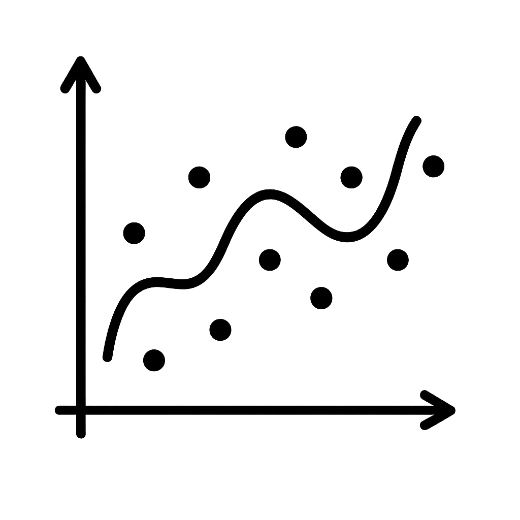
Let's start with a Rorschach Test of sorts:

What does the above elicit in you, what do you feel. If your answer is:

The inherent linearity of it all …

Then we are on the same page. The Red dataset above is numerical statistics from every NBA season (1950-2020) [1] and the Blue dataset is weather data from New York City [2]. I've drawn scatterplots for these datasets based off every permutation of variables and accompanying scatter plots.

What I've tried to capture is a breadth of information, but they share a commonality … linearity. Both datasets, despite their vastly different origins and domains, exhibit patterns where variables co-vary in approximately additive ways. Whether it's player statistics evolving in tandem over decades or atmospheric variables fluctuating in response to seasonal dynamics, the underlying relationships can be described, at least to a first approximation, by linear trends. This shared linearity doesn't imply simplicity, but rather a structural coherence: a kind of statistical grammar that governs how each system organizes and relates its components.

This is a very complicated way of saying Linear Regression is a powerful tool, and can be used to model much of our natural world. However, its important to engage with it in good faith. This writing will attempt to share a couple lessons.

The Context

We will elaborate on Regression Depression in the context of two completely disparate problems:

1. Bitcoin Forecasting: Looking at simple, leakage-safe linear models to predict Bitcoin prices better than naive rules. Using the Cryptocurrency Historical Prices [3] dataset we can reconstruct a daily time series and frame the task as predicting the price at N number of days in the future.
2. Concrete Strength: Predict the compressive strength of concrete based on the concrete's composition and curing age. For our exploration we utilized the Concrete Compressive Strength [4] dataset, our goal is a "formula" that predicts compressive strength (measured in MPa).

Why these two problems specifically? Well for starters these are the most recent problems I've worked on so the challenges of working within each problem-space are still fresh in my head. And also I think these problems provide a good range of context to really explore the full breadth of regression application.

A Note on "Massaging" Data

Massaging data is a very funny term for the process of preparing raw data for analysis. I am not really a fan of massages but their proponents would likely point to nonsensical words like alignment or tension (I really don't believe in massages) and sure those apply to the practice of massaging data as well. But I think of massaging a bit more topologically.

Above is the classic "A Coffee Cup is a Donut" finding from topology, its not really a wow moment but it does get into the essence of homeomorphisms. In topology two things are said to be topologically equivalent through a homeomorphism. These are abstractly defined as some continuous, bijection with an inverse or whatever but when we are talking about shapes (which is what topology is all about) there is a much simpler way.

Can we continuously deform one shape into another without tearing or gluing?

If the answer is yes, then they are topologically equivalent. This is the lens through which I view data preparation: we're continuously deforming our raw data into a shape that our model can work with, stretching and molding it without fundamentally breaking its structure.

Gain Clarity on Multicollinearity

Fundamentally, a regression problem is I have a whole bunch of predictors that I use to find a target the way that I do that is through a function:

$$ \hat{y} = \beta_0 + \beta_1X_1 + \cdots + \beta_nX_n $$

This is simple enough, but what if $X_1$ and $X_2$ are highly correlated? This is the problem of multicollinearity, and it's one of the most insidious issues in linear regression. When predictors are strongly correlated with each other, the regression coefficients become unstable—small changes in the data can lead to wildly different coefficient estimates, making interpretation nearly impossible.

Thinking back to our Bitcoin example we have a dataset of predictors such as:

• Date of observation
• High value on the Date
• Low value on the Date
• Close value on the Date
• Volume of transactions
• Market Cap of Bitcoin on the Date

Immediately we can sniff out that some of these predictors are related to one another based off their description alone … but we can also mathematically qualify this through the Variance Inflation Factor. In simplest terms a VIF is basically designing an auxiliary regression using the predictor $X_i$ as the target, finding a $R^2$ term and using the formula:

$$ VIF_i = \frac{1}{1-R_i^2} $$

Simply put if a predictor variable is able to be modeled as the linear design of the other predictor variables in the dataset it has a high degree of collinearity. Conventionally, we should consider a variable to be collinear if $VIF_i > 10$.

For our Bitcoin dataset, computing the VIF immediately reveals the problem (here we remove the Date field as its kind of of the backbone of our time-series analysis, no value in pointing the finger at it):

Variable	VIF
High	3962.737768
Low	1744.059100
Open	2224.902979
Close	4490.283680
Volume	3.992595
Marketcap	1476.814891

At this point we are basically forced to reconsider our design we can include probably one of High, Low, Open, Close, or Marketcap along with Volume but definitely not more if we want a stable volume. And we can accomplish all this before getting to deep into our model design!

Fill or Kill?

Here's the ugly truth about every dataset that matters … they are ugly. A good datasets is a representation of a real thing and all its nooks and crannies, and any real thing has a certain amount of entropy that manifests itself as noise and more importantly sometimes nothingness.

Missing data is the statistical equivalent of a pothole. Sometimes you can swerve around it, sometimes you need to fill it, and sometimes the best option is to just avoid that road entirely. In regression, how you handle missing values can make or break your model, and the decision between imputation (fill) and deletion (kill) isn't always straightforward.

Let's again examine our Bitcoin dataset to illustrate this dilemma, the dataset itself is unusually well-populated but we have one column Volume that is missing 21 values. In the context of all 2920 rows that isn't an incredible amount but we still need to design a robust strategy. My heuristic involves answering three simple questions:

How Much Data is Missing?

We are only missing around 0.7% of all available datapoints, I don't think its really worth the effort to devise an extra strategy at this point to impute this attribute for likely marginal gains but for posterity we can continue with the other two points.

Why The Data is Missing?

We obviously won't be able to answer this question with 100% certainty, but we can at least make educated guesses. For these datapoints we can see if there is some commonality in the Date field that sheds more insight:

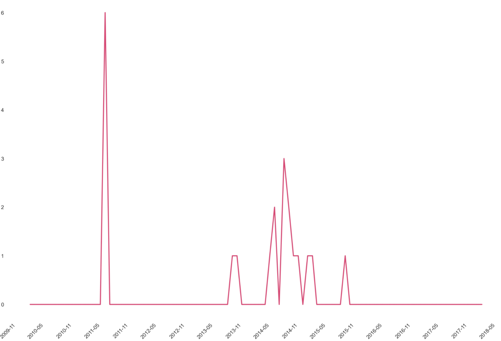
It seems there was one specific period in 2011 contributing to a large amount of the observed missing values (6) wand the rest of the missing datapoints come in an irregular cadence between 2013-2016 the last three years of data collection afterwards were relatively pristine (good job team!).

In this case the systematic nature of the early missing values combined with the scattered later gaps suggests these values are missing completely at random (MCAR) [5] with respect to the actual trading dynamics we're trying to model. Since the missingness isn't informative about Bitcoin's price behavior, deletion won't bias our regression.

Can We Reasonably Infer What It Should Be?

This is the question we must answer to effectively devise a strategy that imputes our data if that is what's required. There are lots of reasonable strategies really depend on the data itself:

• Forward Filling: Insert the last valid observation. This would likely be the best strategy for our missing Volume field as most of the attributes in the Bitcoin dataset are highly dependent on the Date field, so the last valid observation in the time-series is likely a good candidate.
• Measures of Central Tendency: This is better if the specific attribute is stationary (the statistical properties don't really change over time).
• ⚠️ Model-Based Imputation: Use other variables to predict the missing values through a separate regression model. While elegant, this approach may be too smart as it risks introducing circular dependencies in our main analysis.

To Normalize or Standardize?

The question of whether to normalize or standardize your features is one of those decisions that sounds more philosophical than it needs to be, and honestly I get these terms confused all the time. I think in day-to-day conversation just uttering "normalize" or "standardize" makes you sound smart enough that it doesn't really matter if you know the difference … I digress.

Both transformations rescale your features, but they do so in fundamentally different ways:

• normalization (e.g. min-max scaling) squashes values into a bounded range [0,1],
• standardization (e.g. z-score scaling) centers data around zero with unit variance.

I am always a fiend for heuristics so lets design a process:

• So you're building a regression model?
  • Do your features have very different magnitudes?
    • Yes → Use Normalization (scale to 0–1) so no feature dominates the regression.
    • No → Continue.
  • Do you care about comparing coefficients?
    • Yes → Use Standardization (mean = 0, sd = 1) to make coefficients interpretable.
    • No → Continue.
  • Do all features share the same "meaning"?
    • Yes → Use simple Min–Max normalization to express relative share.
    • No → Continue.
  • Default:
    • Use Standardization or apply no correction.

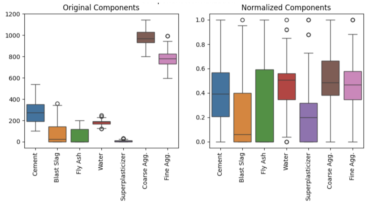
Obviously we loose some "mathematical context" in this flowchart but that's honestly overrated and this is good-enough for most regression based tasks. Looking at our concrete example as defined in the Context section. We had multiple features that basically defined the amount of something you put in to make concrete and they had widely different values (but critically the same unit) normalizing in this context allowed us to assure no specific component dominated the regression.

Eww Is That a Skew?

In the world of data, distributions are rarely polite enough to be perfectly symmetric. Most real-world datasets exhibit some degree of skewness. We observe this as a measure of asymmetry where values bunch up on one side and tail off on the other.

In linear regression, skewed distributions in either your predictors or your response variable can violate the assumption of normally distributed residuals (crazy assumption but hey who am I to judge).

Again looking at our concrete dataset we observed that one field Age had a bit of a skew. To address this the quickest and easiest strategy is usually to apply a log-scale:

⚠️ Note: What we gain in our "assumption of normalicy" we sacrifice in our interprability. The coefficient on log(Age) now represents the effect of a percentage change in age rather than an absolute unit increase, which is a bit less intuitive.

References

1, 2, 3, 4, 5