Fourth and Chaos

The largest draw of professional sports are the players, teams, and stakes. The order of which depends on the sport. One doesn’t need to look farther than the top 10 most watched sports games of the past year to understand that often the content of the game doesn’t matter as much as the context [1]:
.png)
As always NFL is king, but more importantly 8 out of 10 games are attached to the NFL playoffs and the other two fall on Thanksgiving the holiest day of football. This makes sense, because people innately think that bigger means better. The more fanfare and buildup attached to a game like the Superbowl the more likely people are to watch it.
But this fanfare doesn’t always mean that the game is fun to watch. In fact we need not look further than the coveted Superbowl, over the past ten years the Superbowl has on average been decided by more than 11 points [2].
If we strip away the storylines, stakes, and stardom the Superbowl is on average probably more boring than your typical Sunday night game, but I want a way to quantify that, make decisions on which team to watch any given day, and in general capture the how exciting the product on the field or court is irrespective of the fluff surrounding it … cue the Sports Excitement Factor.
I have a very simple strategy to examine the sports excitement factor and it comes down to a funky little chart that most sports degenerates have seen at least one point in our life: The Win Probability Chart.
Let’s take a look at these two games:
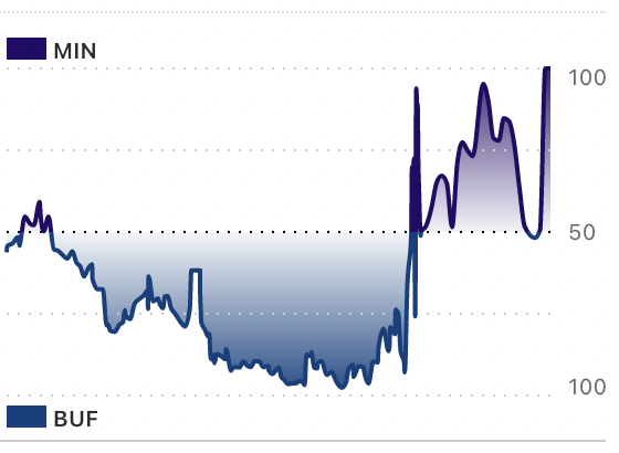
2022 Week 10 NFL Vikings vs. Bills
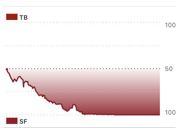
2022 Week 14 NFL 49ers vs. Buccaneers
What was the better game? What was the more exciting game? I think the answer is clear. The most exciting sports games are supposed to ebb and flow like a good story, with twists and turns, surprises and tension, and ultimately a satisfying yet unexpected conclusion.
Before we begin anything we have to construct our in-game win probability model. Unfortunately the folks at ESPN haven’t made their model publicly available, but there is a vast amount of literature on this topic.
Let’s Put Our Model Into Action
With the model “constructed”, we can start our application by taking a simple of random games generated by our model. All games used in our analysis are going to be from the 2022 NFL season.
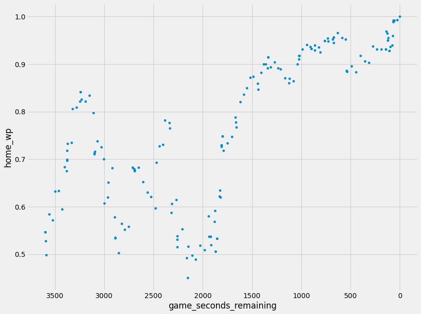
Week 12 - Green Bay @ Philadelphia (33-40)
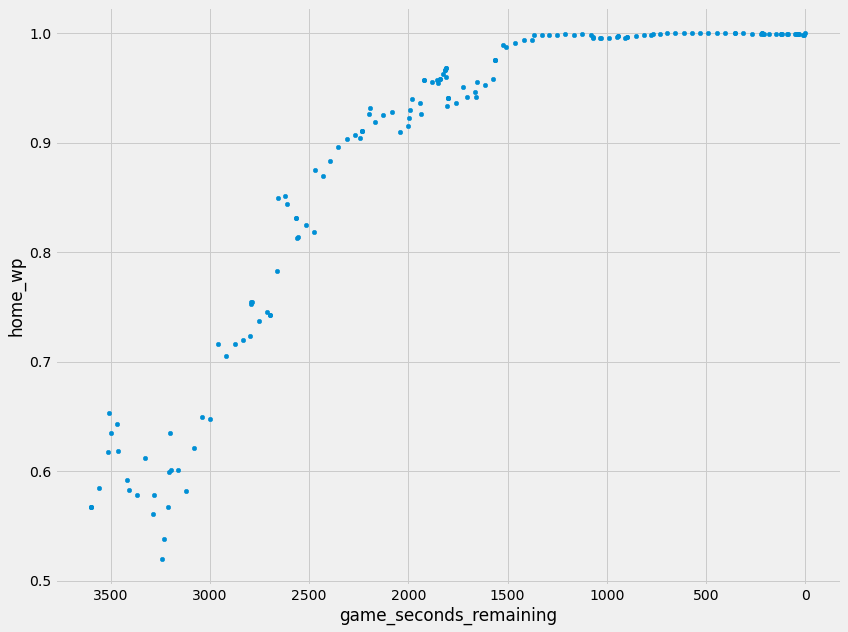
Week 8 - Las Vegas @ New Orleans (24-0)
The essence of what we are looking for is there, now it’s just time to throw some numbers around and see what sticks.
Quantifying It All
The graph is nice but it doesn’t provide anything quantitative to compare, sort, and assess. Instead we need to figure out a way to project the figures above down into a single number. Here are a couple of ideas to quantify it all:
- Time Spent in “Danger Zone”: Lets say the danger zone is a game that is at about a 50% win probability for either team with a margin of error of about 5%, we can then look for the portion of a game that’s in this zone
- Big Movements: Looking for large changes in the win probability, maybe we can define this as within a minute if the win probability changes more than 20%. This would usually indicate a turnover or big offensive play. In other words “exciting”.
- Eccentricity: This one is a bit harder to define but how about a way of saying how weird the general essence of a win probability graph is. Or in other words how hard it is to capture with mathematical functions?
The Danger Zone is pretty easy to numerate:
$$ d = \frac{45 \leq obs_i \leq 55}{obs} $$
Where obs is the number of observation points, now one might note that this isn’t exactly a perfect comparison because points are not evenly distributed, but it should be good enough. However one thing that we need to to take a more critical look at is weighing these metrics towards the end of the game. A tie game in the first quarter means much less than a tie game at the end of the fourth.
$$ d = \frac{\Sigma_{i=0}^{N} (\ln(i + 1) + 1) \cdot(45 \leq obs_i \leq 55)}{N} $$
I don’t pretend to be a mathematician in any sort of the word, but the approach I’m suggesting is that we weigh observations using a log function to naturally mimic the gradient within the “stakes” of a game. We are using the log as a factor multiplied to our binary observations.
Big movements, like the danger zone, is in principal pretty easy to calculate:
$$ m = \frac{|obs_{i} - obs_{i + 1}| \geq 5 }{obs} $$
Same ingredients different meal, here we are simply looking at each observation along with the previous figuring out if the difference is larger than some arbitrary threshold which in this case is 5%. In this case we can similarly apply the log factor to weigh observations towards the end of the game.
I’m going to try something different for eccentricity, and it starts with perhaps the nerdiest assumption I’ve ever made. So nerdy that I’m going to put it in a quote card distinct from the rest of my writing in order to salvage the dignity of my prose.
“Let’s assume any football win probability can be modeled as a polynomial function with an arbitrary amount of terms”
And I’m going to make another assumption this time about you the audience. If football win probability can be modeled by a polynomial function we want more terms not less. A linear win probability sounds extremely boring, however if we crank those numbers up to perhaps a nonic (a degree of 9) we start cooking.
As a thought exercise what if we approximate the polynomial representation of the win probability graph using a polynomial with degree equivalent to 50% of the total number of observations 10 (for computational reasons).
$$ \set{obs_0 \cdots obs_N} \rightarrow β_1x^{\frac{N}{2}} + β_2x^{\frac{N}{2}-1} + \cdots +β_{\frac{N}{2}}x^0 = f(n) $$
Again, I don’t claim to be a mathematician in any sort of the word, but the general idea is I want to transform a random subset of the observations into a polynomial function representing the win probability. That transformation process isn’t detailed in depth, but we would be using polynomial regression.
Now from there we can simply reference our observations against the function like so:
$$ e = \Sigma_{i = 0}^{N} |f(i) - obs_i| $$
Akin to the other metrics we’ve calculated, a larger value is good in the larger scheme of finding an exciting game. Well that’s enough math for the day, lets delve into the real meat and potatoes of what we are after and construct our excitement algorithm.
Weights and Biases
Well now with all algorithms in place, what do we actually do with these three numbers. Well the simple answer is to just add them up together:
$$ excitement = \beta_0 (danger) + \beta_1 (movement) +\beta_2 (eccentricity) $$
After computing all the values for the 2023-2024 NFL season we are left with data that looks like this:
game_id |
danger_zone |
big_movements |
eccentricity |
excitement |
|---|---|---|---|---|
| 2023_01_ARI_WAS | 1.0629 | 0.5632 | 0.2961 | 1.9222 |
| 2023_01_BUF_NYJ | 1.0585 | 1.0630 | 0.3446 | 2.4661 |
| 2023_01_CAR_ATL | 1.4922 | 0.6228 | 0.1732 | 2.2882 |
| 2023_01_CIN_CLE | 0.0712 | 0.2938 | 0.1542 | 0.5192 |
| . . . | . . . | . . . | . . . | . . . |
And pretty quickly we can say the most exciting game of the 2023-2024 season was the … drumroll please … 2023_14_MIN_LV with a score of 4.0948 or in human terms:
NFL Week 14 Game Recap: Minnesota Vikings 3, Las Vegas Raiders 0
Yeah, that’s not really what we are after - a total of three points were scored in this close, or in NFL terms one paltry field goal. Yes this game was in the danger_zone for quite some time, mostly by virtue of Josh Dobbs passing for 63 yards [3]. This was so close to what we were looking for but not quite there. In fact, if we look further down the list at the second most “exciting” game we find 2023_01_BUF_NYJ (3.7266) better known as the game that Aaron Rodgers blew out his Achilles in his first 5 minutes playing with the Jets:
NFL Week 1 Game Recap: New York Jets 22, Buffalo Bills 16
That was a pretty exciting game independent of the injury. It was a back and forth game where the Jets emerged victorious in overtime … so that proves a little merit to our model.
Remember those funny little beta symbols that I wrote down - let’s try using those. What we are actually after is an adequate weighting of our three parameters that emphasizes the correct attributes according to their importance in the excitement of a game. How we achieve the system of carefully tuning our weighting is through Linear Regression [4], how we put this into action is a little bit more complicated.
How To Overcomplicate a Problem
Obviously to perform a linear regression or any model tuning we need something to assess our weights against. That something should be an equivalence of the problem we are exploring even if not 11:1. In that case we are looking for some quantity that tells us how exciting a game is to serve as our training data - sound familiar? Well that’s the whole essence of our problem? We can’t use TV viewership for reasons discussed in the prologue, so we have to get creative with how to attack this problem.
Well we could do this and overcomplicate what in essence is a simple(r) problem, or … we could trust on good authority that Emily Iannaconi from NBC Sports does a pretty good job in her ranking of most exciting regular season games and take it from there [5]. The data in the linked article accounts for a hodgepodge of games from the 2022-2023 season as well as the 2023-2024 season so we will have to expand our dataset by a season.
As for scoring the data we can arbitrarily say that the most exciting game is a 100 and the second, third, and beyond most exciting games have a score on a log scale as described in Zipf’s Law [6]. Or more succinctly for all game rankings r in the ground-truth dataset:
$$ \text{excitement}(r) = \frac{100}{r} $$
In total we have 10 games to quantify and their manually assigned “excitement” ratings are as follows:
game_id |
excitement |
|---|---|
| 2022_22_KC_PHI | 100 |
| 2023_12_BUF_PHI | 50 |
| 2023_14_LA_BA | 33.33 |
| 2022_19_LAC_JAX | 25 |
| 2023_15_PHI_SEA | 20 |
| 2022_21_CIN_KC | 16.67 |
| 2023_01_BUF_NYJ | 14.28 |
| 2023_04_WAS_PHI | 12.5 |
| 2023_01_DET_KC | 11.11 |
| 2023_11_PHI_KC | 10 |
And after a bit of data cleaning and a simple linear regression model we are left with a final formula of excitement as:
$$ \text{excitement} = -13.59837102 \cdot \text{dz} -38.03332362 \cdot \text{bm} + 174.61538549 \cdot \text{ec} $$
Well, that’s rather interesting - it almost seems like excitement is strictly defined by eccentricity and the danger zone or big movements of a game don’t really add much value. Usually at this step if we have a model that looks like this we would reconsider our parameters, retrain, and live to fight another day. Instead, I’m going to do none of that and trudge forward.
Putting “Excitement” In Context
The reason I’m so rash to accept our model and move on is that I’m much more interested in what we can do with a quantitative metric of excitement and less interested in how we got there (this is fundamentally the wrong approach, please do not follow this philosophy in any aspect of your life but its almost 1:00AM and I really want to finish writing this).
We can begin by revisiting our esteemed title of “Most Exciting Game of The 2024” Season to find … 2023_07_BUF_NE which was frankly a pretty exciting game. I could sell it to you, or I could simply show the win-probability chart:
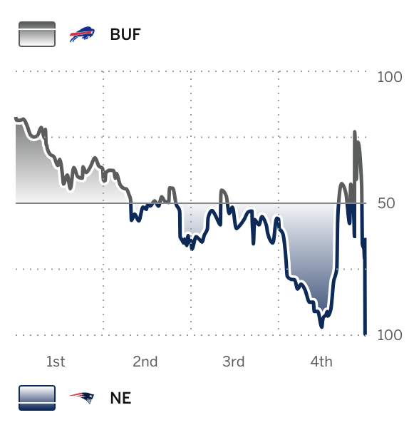
We are slowly discovering the value of our quantitative approach to excitement. First of all - it doesn’t matter that this game was a quarterback duel between Josh Allen and Mac Jones in Week 7, all that matters is the raw datapoints. With that in mind lets generate some results. Starting with something I had a vested personal curiosity in Average Excitement by Week:
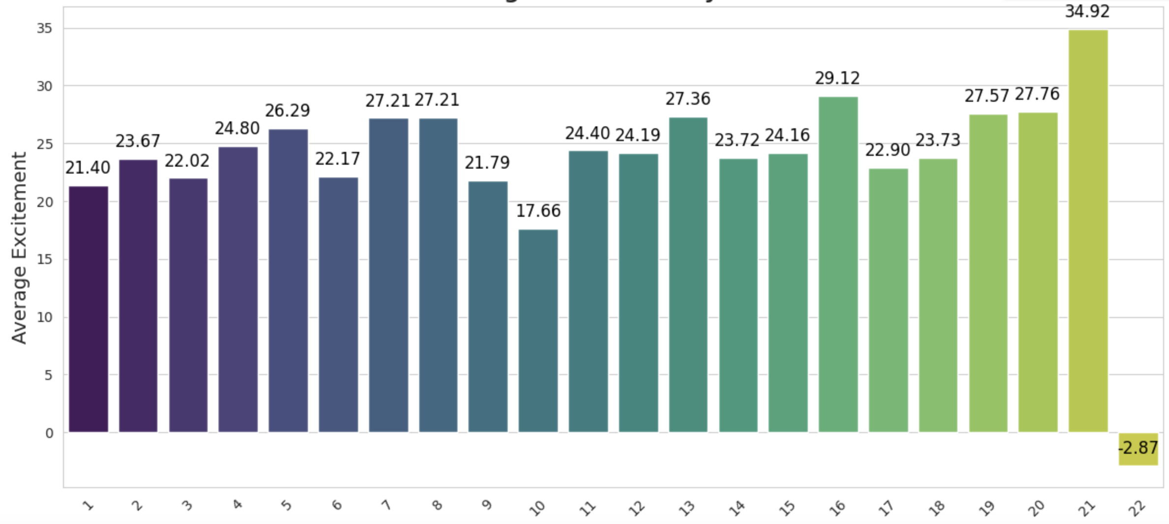
Initially I though that the NFL season on balance started out pretty dull with excitement ramping up towards the end of the season but instead it looks like excitement is pretty well balanced throughout the weeks. Next, another personally curiosity was Share of Excitement by Team. We know certain teams command an unfair share of the media’s attention but when we boil the numbers which teams share the largest wedge of the leagues excitement product:
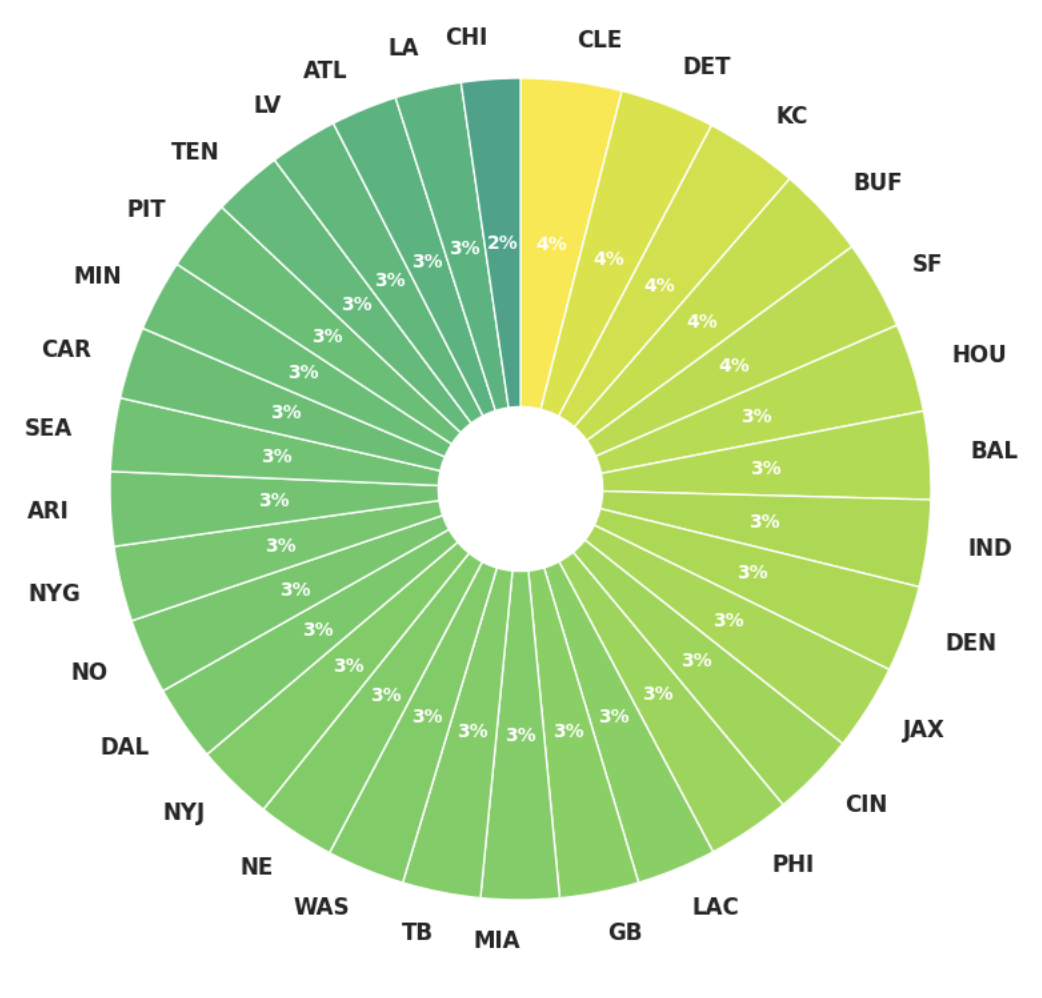
There really isn’t much differentiation between teams which is probably a good thing for the television product but we can see slight bias towards a couple of teams: KC, DET, BUF, SF, and CLE. The commonality between most of those teams is that they are just on-balance good teams who probably compete in lots of high-leverage games, but the addition of Cleveland on that list does pique some curiosity.
Wrapping Up
While our meandering adventure might not revolutionize how we watch football, it's given us a way to justify why we spend our Sundays glued to RedZone even if its a 1PM Buccaneers-Saints game. Excitement is not driven by the names, stakes, or fanfare. Sometimes pure, unadulterated chaos rules supreme.
I find it kind of symbolic that out of every variable “Eccentricity” is the one weighted so heavily by a Linear Regression; definitely out of the formulas I created it felt the most like quack-science, but maybe the speaks to a more philosophical point about this entire exploration. We don’t really know what makes Football click in the brain of the average American Audience - yes the detractors may point to nationalism, brutality, etc. but I don’t really buy that argument. There is just something so appealing about watching a symphony of crashes and bumps play out over 60 minutes. Any model of Football will never provide the predictive capabilities we covet, but at least an excitement model comes one step closer to qualifying why we love this game oh-so much.